Info to beginners:
This tutorial concerns a more “advanced” usage of SciQLop. If you are a beginner with SciQLop, you should probably start looking at the Basic Plotting Workflow and how to create Catalogs.
In the Basic Plotting Workflow tutorial, we have plotted data that is accessible from the product tree and proposed by web services. Although tens of thousands of products are readily available in there, you may quickly feel limited as your research workflow will sooner or later require plotting quantities that are more complex than data proposed by mission servers.
For instance, you may want to plot, along with “regular” data from servers:
- the result of a mathematical expression such as the local plasma frequency, or the firehose or mirror instability threshold, or the components of the local velocity
- the magnetic field components, transformed into another coordinate system
- a pitch angle spectrogram for a specific energy band from the distribution function
- etc.
In this tutorial we will discover a great feature of SciQLop that will allow you to plot basically anything you want, provided you can write a little bit of Python.
What is a virtual product?
A virtual product is like a “normal” data product you get from the product tree, but instead comes from running a user defined Python function. It is very simple to make a virtual product and interact with it:
- define a Python function that takes two arguments
startandstop, the time interval for which the product is computed
def mirror_mode_threshold(start, stop):
    my_prod = ...  # compute your product the way you want
return my_prod- let SciQLop know about your function by creating a virtual product:
create_virtual_product("mms_vprods/mms1/mirror",
                       mirror_mode_threshold,
                       VirtualProductType.Scalar,
                       labels=["Mirror mode threshold"])
don’t worry we will explain this in more details below. Essentially this will add a product in the product tree at the path mms_vprods/mms1/mirror, which you can now drag and drop in a plot panel as any other product. SciQLop will call your function passing the window’s time interval as argument and display the result. It’s as simple as that.
Open a Jupyter notebook
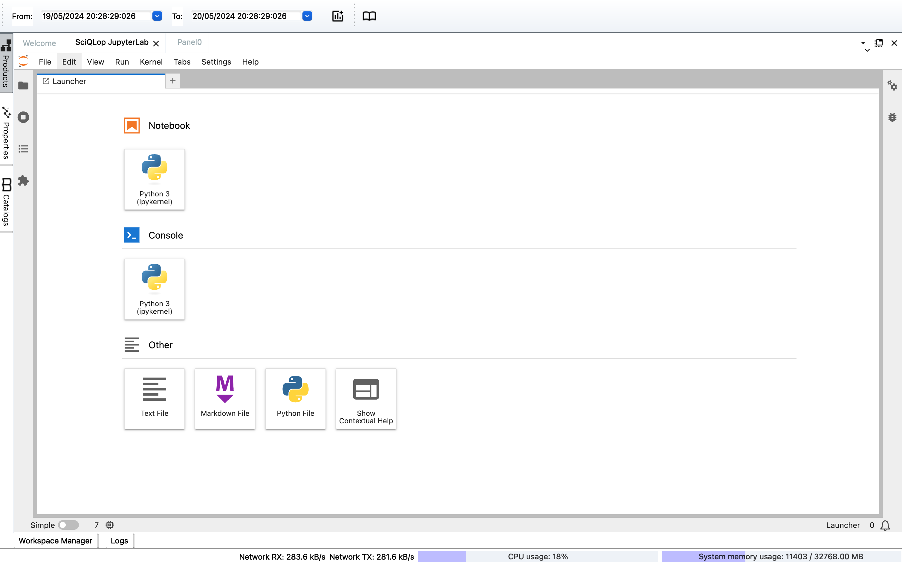
Jupyter notebooks are embedded in SciQLop to let you interact with the software. Open JupyterLab from Tools › Open JupyterLab, then click on “Python 3 (ipykernel)” under “Notebook” to open a new notebook. This notebook runs inside SciQLop, so it can drive it.
Mirror mode instability threshold
Let’s investigate the mirror mode instability with SciQLop. The formula is:
with
We aim at plotting as a regular product along with other products.
In our notebook let’s first import SciQLop packages for virtual product definition
from SciQLop.user_api.virtual_products import create_virtual_product, VirtualProductTypethen import Speasy to download and manipulate data, as well as SciPy:
from speasy import SpeasyVariable
from speasy.signal.resampling import interpolate
import speasy as spz
import scipy.constants as cst
here comes our mirror mode threshold function:
def mirror_mode_threshold(start_time: float, stop_time: float) -> SpeasyVariable | None:
    mms1_products = spz.inventories.data_tree.cda.MMS.MMS1
    products = [mms1_products.DIS.MMS1_FPI_FAST_L2_DIS_MOMS.mms1_dis_temppara_fast,
                mms1_products.DIS.MMS1_FPI_FAST_L2_DIS_MOMS.mms1_dis_tempperp_fast,
                mms1_products.FGM.MMS1_FGM_SRVY_L2.mms1_fgm_b_gse_srvy_l2,
                mms1_products.DIS.MMS1_FPI_FAST_L2_DIS_MOMS.mms1_dis_numberdensity_fast]

    tpara, tperp, b, n = spz.get_data(products, start_time, stop_time)

    anisotropy = tperp / tpara
    Pperp = tperp * n * 1e6
    b = interpolate(tperp, b)
    betaperp = Pperp * cst.mu_0 * cst.e * 2 / (b["Bt"] * 1e-9) ** 2
    mirror = betaperp * (anisotropy - 1)
    return mirror
in this function we simply:
- ask Speasy to download all raw products from CDAWeb for the time interval SciQLop will provide to the function
- compute the mirror mode formula given above. Note this requires interpolating the temperature onto the magnetic field timestamps, which Speasy allows you to do easily
- return the
mirrorvariable
Then comes our virtual product definition already given above:
mirror_mode_threshold_vp = create_virtual_product("mms_vprods/mms1/mirror", mirror_mode_threshold,
                                                  VirtualProductType.Scalar, labels=["Mirror mode threshold"])
From now on, SciQLop knows about our virtual product. It is registered in the product tree at the path mms_vprods/mms1/mirror. The arguments to create_virtual_product are:
"mms_vprods/mms1/mirror": the path in the product tree where the virtual product will be accessiblemirror_mode_threshold: the Python function SciQLop needs to call to compute this virtual productVirtualProductType.Scalar: the type of virtual product, here it is a scalar but you can also compute vectors (VirtualProductType.Vector), any number of components (VirtualProductType.MultiComponent) or spectrograms (VirtualProductType.Spectrogram)labels=["Mirror mode threshold"]: the legend SciQLop will show on the plot. A scalar needs one label, a vector three, a multi-component product one per component. A spectrogram takes none.
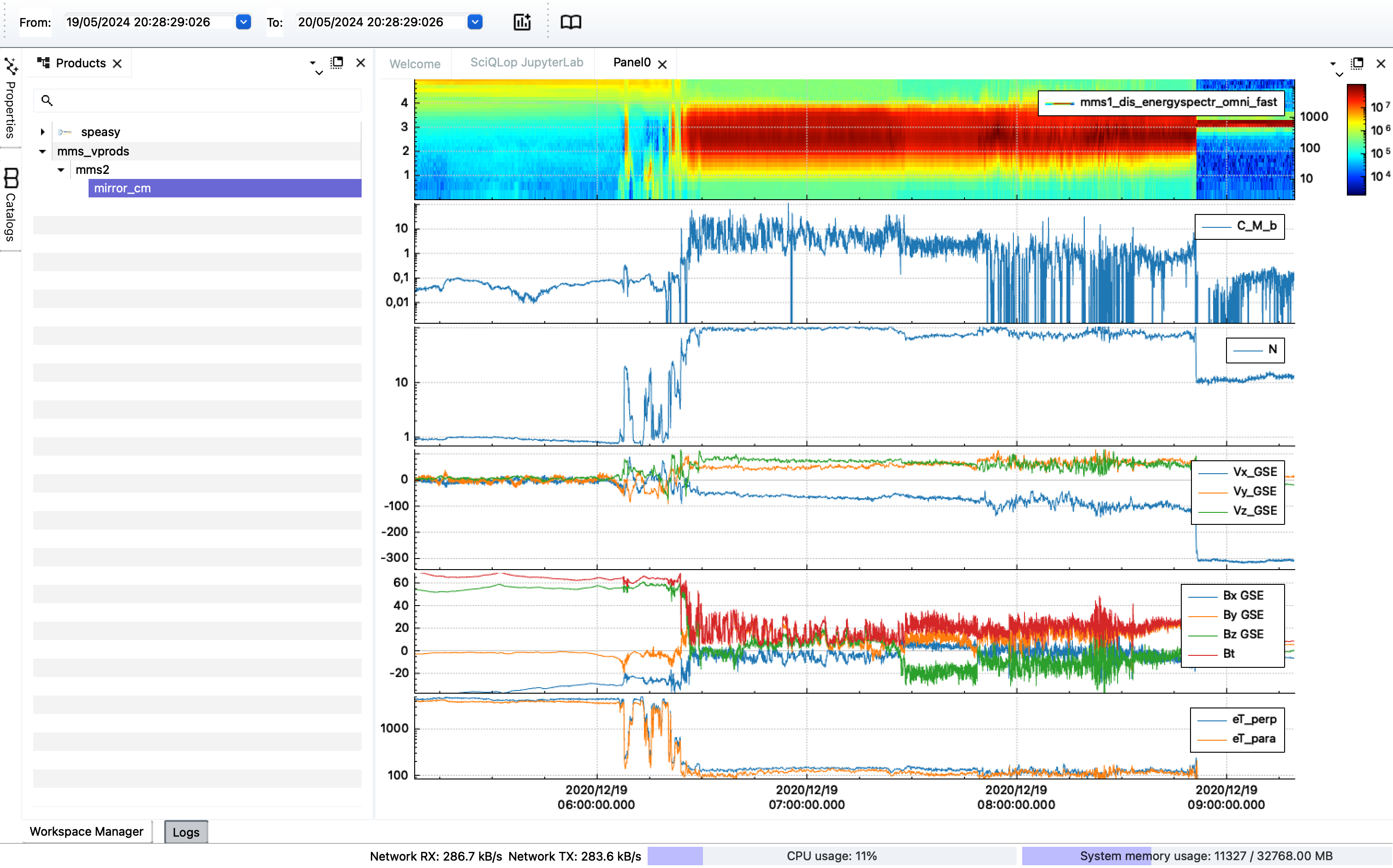
The screenshot below shows, on the left in the product tree, the virtual product we have created. It has been drag-and-dropped in the second plot from the top in the current plot panel in the following screenshot.
Let SciQLop fetch the inputs
Our function fetches its own data with spz.get_data. You can instead declare the inputs in its signature. Annotate a parameter with Depends("<product path>"). SciQLop then fetches that product over the requested interval and passes it in.
from typing import Annotated
from SciQLop.user_api.virtual_products import Depends

MOMS = "speasy//cda//MMS//MMS1//DIS//MMS1_FPI_FAST_L2_DIS_MOMS"
FGM = "speasy//cda//MMS//MMS1//FGM//MMS1_FGM_SRVY_L2"

def mirror_dep(start: float, stop: float,
               tpara: Annotated[SpeasyVariable, Depends(MOMS + "//mms1_dis_temppara_fast")],
               tperp: Annotated[SpeasyVariable, Depends(MOMS + "//mms1_dis_tempperp_fast")],
               n: Annotated[SpeasyVariable, Depends(MOMS + "//mms1_dis_numberdensity_fast")],
               b: Annotated[SpeasyVariable, Depends(FGM + "//mms1_fgm_b_gse_srvy_l2", pad=30.0)],
               ) -> SpeasyVariable | None:
    b = interpolate(tperp, b)
    betaperp = tperp * n * 1e6 * cst.mu_0 * cst.e * 2 / (b["Bt"] * 1e-9) ** 2
    return betaperp * (tperp / tpara - 1)

create_virtual_product("mms_vprods/mms1/mirror_dep", mirror_dep,
                       VirtualProductType.Scalar, labels=["Mirror mode threshold"])
A few details:
- The paths are product-tree paths, with
//between levels, like the ones you drag from the tree. pad=30.0widens the fetch by 30 s on each side. Here it keeps the interpolation backed by data at both edges of the window. It also takes atimedelta.- When an input has no data, SciQLop skips the call and the product shows nothing.
Going further
- The
%%vpcell magic lets you define a virtual product directly from a notebook cell, with hot reload when you re-run the cell. A return annotation such as-> Scalar["Mirror mode threshold"]or-> Vector["Bx", "By", "Bz"]sets the type and the labels.- Since v0.12, keyword arguments with default values on your callback become interactive knobs (sliders, spinboxes, choices). They show in the Adjustable inputs section of the Properties panel — perfect for thresholds and tunable parameters.
- Both are demonstrated in the tutorial notebooks bundled with SciQLop (see the welcome page).