Info to beginners:
This tutorial concerns a more “advanced” usage of SciQLop. If you are a beginner with SciQLop, you should probably start looking at the Basic Plotting Workflow and how to create Catalogs.
Why templates?
The Basic Plotting Workflow allows you to easily plot data with SciQLop by drag-and-dropping products from the product tree onto a plot panel. Although this is already way simpler than in most existing tools, this way of creating plots will quickly become a limitation to your workflow.
As you do your data exploration or analysis, you will very probably often want to look at the same data products, in the same order, with the same styles, colors, etc. Doing all that with your mouse, each time you re-open SciQLop, is needlessly long.
SciQLop offers two complementary answers:
- Panel templates (since v0.12): save any panel as a named template and re-instantiate it in one click.
- Scripting your routine plots with the Python API.
Panel templates
Once you have built a panel you like — by drag-and-drop, scripting, or both — save it as a template. With the mouse, right-click the panel and choose Panel templates › Save as template…. From Python:
p.save_template("my_mms_overview")A template stores the products of each plot, in order, with their adjustable inputs. It also keeps the axis scales and ranges, and the time range. Curve colours and styles are not kept. Only products from the product tree are saved: data you plotted from arrays or a function is skipped.
Saved templates appear in the Templates section of the welcome page. Click a card to open the template in a new panel. Right-click it to rename or delete it.
Templates are plain JSON files. To share one, right-click the panel and choose Panel templates › Export template…, which also writes YAML. Your colleague imports it with the Import… card of the welcome page. A panel opened from a template gets an Update template entry in the same menu, to save your changes back.
The file format, and how templates relate to Speasy proxy share links, is described in Template format.
Scripting a routine plot
To obtain the following screenshot
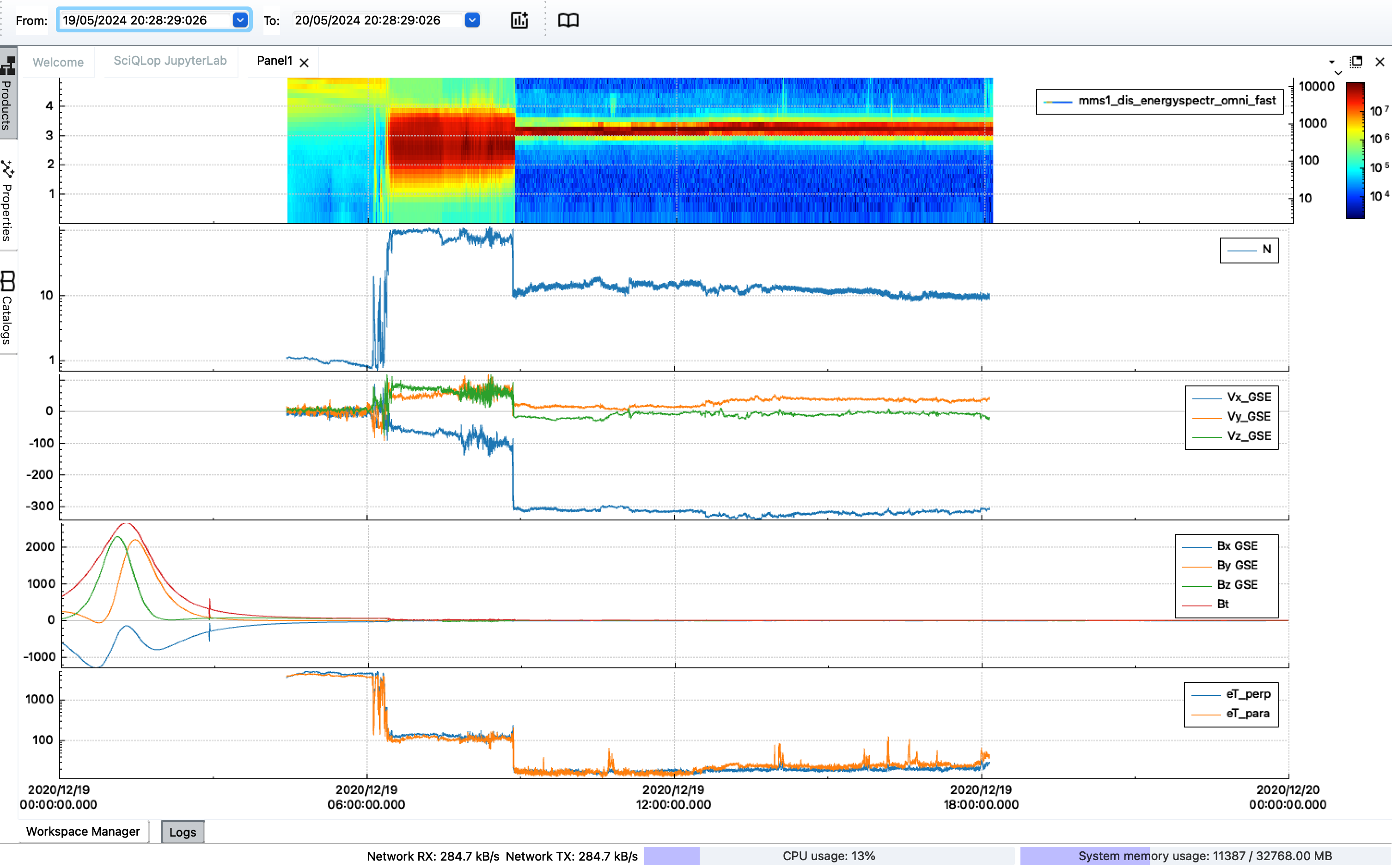
simply write this in a Jupyter notebook embedded in SciQLop.
First import all plotting routines offered by SciQLop:
from SciQLop.user_api.plot import *then create a plot panel (this is the Python equivalent of the button on the top of the SciQLop window), set its time range, and use the returned plot panel handle (p) to make plots by calling the method plot:
p = create_plot_panel()
p.time_range = TimeRange("2020-12-19", "2020-12-20")
p.plot("speasy//cda//MMS//MMS1//DIS//MMS1_FPI_FAST_L2_DIS_MOMS//mms1_dis_energyspectr_omni_fast")
p.plot("speasy//cda//MMS//MMS1//DIS//MMS1_FPI_FAST_L2_DIS_MOMS//mms1_dis_numberdensity_fast")
p.plot("speasy//cda//MMS//MMS1//DIS//MMS1_FPI_FAST_L2_DIS_MOMS//mms1_dis_bulkv_gse_fast")
p.plot("speasy//cda//MMS//MMS1//FGM//MMS1_FGM_SRVY_L2//mms1_fgm_b_gse_srvy_l2")
p.plot("speasy//cda//MMS//MMS1//DIS//MMS1_FPI_FAST_L2_DIS_MOMS//mms1_dis_tempperp_fast")
Get the product path easily
Note the name of each product is a long string that is tedious to write… but you can get it by drag-and-dropping the product from the product tree to the notebook cell. Easy!
Then grab the last plot (index 4 in the panel plots p.plots list) where the perpendicular temperature is represented, and plot the parallel temperature on top.
p.plots[4].plot("speasy//cda//MMS//MMS1//DIS//MMS1_FPI_FAST_L2_DIS_MOMS//mms1_dis_temppara_fast")Finally, set plots indexed 1 and 4 (density and temperatures) to have a log Y scale.
p.plots[1].y_scale_type = ScaleType.Logarithmic
p.plots[4].y_scale_type = ScaleType.Logarithmic
And of course, you can now save the result as a template — best of both worlds:
p.save_template("mms_moments_overview")