Virtual products

A virtual product is a Python function that SciQLop calls for the visible time range. It shows in the Products tree under the path you choose, and it plots like any other product. virtual products walks through a full example.

`create_virtual_product`

vp = create_virtual_product(path, callback, product_type, labels=None,
                            debug=False, cachable=False,
                            knobs_model=None, knobs_kwarg_name="knobs",
                            display_name=None)

Parameter	Meaning
`path`	Where it goes in the Products tree, like `"my_products//mms1//b_total"`.
`callback`	Your function `f(start, stop, ...)`.
`product_type`	A `VirtualProductType`. See the table below.
`labels`	Component names. How many depends on the type.
`debug`	`True` prints the callback’s stack traces. Handy while writing it.
`cachable`	`True` tells SciQLop the function always returns the same data for the same range, so results can be cached.
`knobs_model`	A Pydantic model whose fields become knobs. The instance is passed as `knobs_kwarg_name`.
`display_name`	Name shown in the tree and on the plot. Used by spectrograms only in v0.13.1; by every type in the next release.

`VirtualProductType`	`labels`	Callback returns
`Scalar`	exactly 1	`(t, y)` with `y` of shape `(N,)` or `(N, 1)`, or a `SpeasyVariable`
`Vector`	exactly 3	`(t, y)` with `y` of shape `(N, 3)`, or a `SpeasyVariable`
`MultiComponent`	any number, at least 1	`(t, y)` with `y` of shape `(N, n)`, or a `SpeasyVariable`
`Spectrogram`	ignored	`(t, y, z)` or a 2-D `SpeasyVariable`

Next release

labels can come from the callback’s return annotation. With def f(start, stop) -> Scalar["|B|^2"], create_virtual_product(path, f, VirtualProductType.Scalar) needs no labels=. An explicit labels= still wins.

The result is a VirtualProduct. Pass it anywhere a product path is accepted: p.plot(vp). Its path and product_type are readable. Registering the same path again replaces the old product.

import numpy as np
import speasy as spz
from speasy.products import SpeasyVariable
from SciQLop.user_api.virtual_products import create_virtual_product, VirtualProductType
 
def b_total(start: float, stop: float) -> SpeasyVariable | None:
    b = spz.get_data("cda/MMS1_FGM_SRVY_L2/mms1_fgm_b_gse_srvy_l2", start, stop)
    if b is None:
        return None
    return b["Bt"]
 
b_total_vp = create_virtual_product("my_products//mms1//b_total", b_total,
                                    VirtualProductType.Scalar, labels=["|B|"], cachable=True)
p.plot(b_total_vp)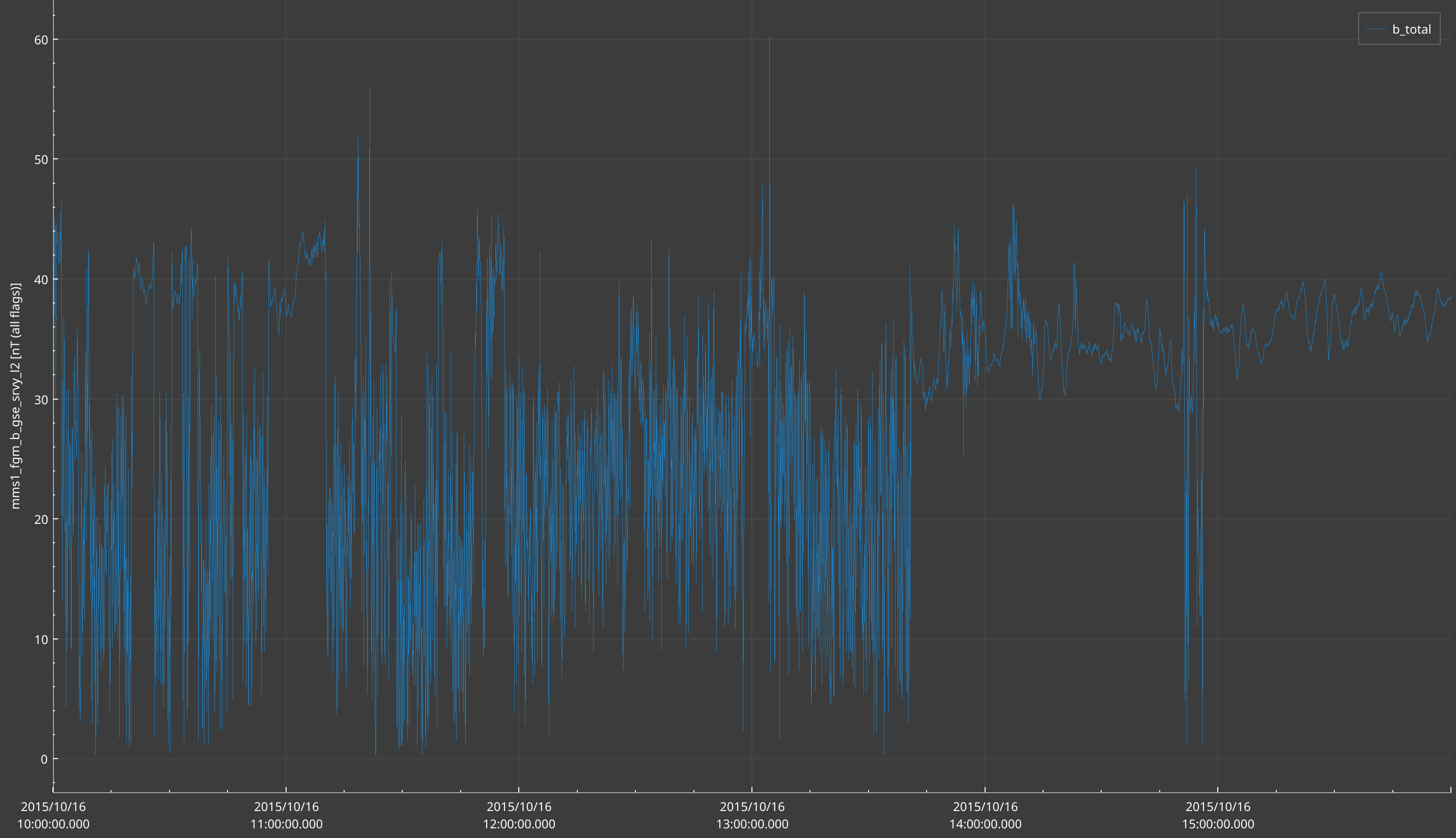

The callback contract

SciQLop calls the function with start and stop, the range to compute.
Their type follows your annotations. float (or no annotation) gives epoch seconds. datetime gives UTC datetimes. np.datetime64 gives datetime64[ns].
The function returns a SpeasyVariable, a tuple of arrays, or None for “no data”.
The time axis you return can be datetime64 or epoch seconds as float64.
The call runs on a worker thread, not the GUI thread. Compute and return data. Don’t drive the GUI from there.

Returning a SpeasyVariable is the better choice. Its units, axis labels and scale reach the plot for free. Do the maths on the SpeasyVariable itself, not on .values, so the time axis and units stay attached.

Inputs with `Depends`

A callback can declare the products it needs. SciQLop fetches them for the same range and passes them in.

from typing import Annotated
from speasy.products import SpeasyVariable
from SciQLop.user_api.virtual_products import Depends, create_virtual_product, VirtualProductType
 
FGM_DS = "speasy//cda//MMS//MMS1//FGM//MMS1_FGM_SRVY_L2"
 
def b_squared(start: float, stop: float,
              b: Annotated[SpeasyVariable, Depends(FGM_DS + "//mms1_fgm_b_gse_srvy_l2", pad=30.0)],
              ) -> SpeasyVariable | None:
    return None if b is None else b["Bt"] ** 2
 
create_virtual_product("my_products//mms1//b_squared", b_squared,
                       VirtualProductType.Scalar, labels=["|B|^2"])

The target can be a product path, a VirtualProduct, or a function f(start, stop).
pad widens the fetched range on both sides, in seconds or as a timedelta.
Dependencies are always resolved with epoch-second bounds.

Knobs: parameters you can tune

Keyword arguments with a default become knobs. You tune them in the inspector, and the product is recomputed. See Knobs for the full list.

from typing import Annotated, Literal
from SciQLop.user_api.knobs import Knob
 
COLUMN = {"Bx": 0, "By": 1, "Bz": 2}
 
def smoothed(start: float, stop: float,
             window: Annotated[int, Knob(min=1, max=200, step=1, label="Window", unit="samples")] = 10,
             component: Literal["Bx", "By", "Bz"] = "Bx"):
    b = spz.get_data("cda/MMS1_FGM_SRVY_L2/mms1_fgm_b_gse_srvy_l2", start, stop)
    if b is None:
        return None
    y = np.convolve(b.values[:, COLUMN[component]], np.ones(window) / window, mode="same")
    return b.time, y
 
create_virtual_product("my_products//mms1//b_smoothed", smoothed,
                       VirtualProductType.Scalar, labels=["B smoothed"])

The names start, stop and data are reserved and never become knobs.

From a notebook cell: `%%vp`

The %%vp cell magic registers the function defined in the cell. Re-running the cell hot-reloads it: open plots use the new code on their next fetch.

%%vp --path "my_products/sine" --debug --start "2020-01-01" --stop "2020-01-02"
import numpy as np
 
def sine(start: float, stop: float, frequency: float = 0.01) -> Scalar["sin"]:
    t = np.arange(start, stop, 5.0)
    return t, np.sin(2 * np.pi * frequency * (t - start))

Scalar, Vector, MultiComponent and Spectrogram are injected into the cell. Annotate the return with them: -> Vector["Bx", "By", "Bz"].
Without an annotation, the magic calls the function once and guesses the type from the result.
The cell must define exactly one public function. Name helpers with a leading _.
Options: --path (defaults to the function name), --debug (opens a debug panel), --start / --stop (the test range), --cachable.

Other helpers

Name	What it does
`VirtualScalar`, `VirtualVector`, `VirtualMultiComponent`, `VirtualSpectrogram`	The classes behind `create_virtual_product`. Their constructors also take `out_of_process=True`.
`SciQLop.user_api.virtual_products.fspeasy`	`get_data`, `lift`, `pipeline`: a `speasy.get_data` that returns `Something`/`Nothing` instead of `None`, for chained pipelines.

Next release

list_virtual_products() returns the // paths of every registered virtual product.

A virtual product can colour its line by a scalar. Return Colored(data, color=c) with one value per sample, and register with create_virtual_product(..., colored=True, color_label="|B| (nT)", color_gradient="thermal"). In a %%vp cell, annotate -> Colored[Vector["X", "Y", "Z"]]. Not for spectrograms.

cachable=True products fetch half a view extra on each side, so small pans need no new fetch.

%%vp understands return annotations written under from __future__ import annotations.

Knobs

Knobs are tunable parameters of virtual products and annotation layers. SciQLop builds them from the callback’s keyword arguments.

Keyword argument	Knob	Inspector widget
`n: int = 10`	`IntKnob`	spin box
`x: float = 0.5`	`FloatKnob`	spin box
`flag: bool = True`	`BoolKnob`	check box
`mode: Literal["a", "b"] = "a"`	`ChoiceKnob`	drop-down
`name: str = "x"`	`StringKnob`	text field
`w: SciQLopPlotRange = SciQLopPlotRange(0.3, 0.7)`	`TimeRangeKnob`	a draggable span on the plot
`level: Annotated[float, Knob(widget="hline")] = 1.0`	`ThresholdKnob`	a draggable horizontal line

Wrap the type in Annotated[..., Knob(...)] to add details:

Knob(min=None, max=None, step=None, label="", unit="", description="",
     apply="live", choices=None, pattern="", widget="", color="")

Field	Meaning
`min`, `max`, `step`	Bounds and increment.
`label`, `unit`, `description`	Text shown in the inspector.
`apply`	`"live"` recomputes on every change. `"manual"` waits for you to apply.
`choices`	A list of values, or `(label, value)` pairs, for a drop-down.
`pattern`	A regular expression a string knob must match.
`widget`	`"vspan"` for a time span, `"hline"` for a horizontal line.
`color`	Colour of the span or line on the plot.

A time-span knob given a default between 0 and 1, like SciQLopPlotRange(0.3, 0.7), starts as that fraction of the visible range. Import SciQLopPlotRange from SciQLop.user_api.knobs.

DatetimeKnob and StringListKnob are exported too, but only catalog attribute editing uses them. A callback’s keyword arguments never produce them.

Next release

Annotated[float, Knob(widget="vline")] = 0.5 is a time cursor: a draggable vertical line. The callback gets its time in epoch seconds. A default between 0 and 1 is a fraction of the visible range.

Knob(scope="plot") keeps a span or cursor on the product’s own plot. The default, "panel", draws it on every plot of the panel.

SciQLop

Explorer

Virtual products and knobs

Virtual products

`create_virtual_product`

The callback contract

Inputs with `Depends`

Knobs: parameters you can tune

From a notebook cell: `%%vp`

Other helpers

Knobs

Table of Contents

SciQLop

Explorer

Virtual products and knobs

Virtual products

create_virtual_product

The callback contract

Inputs with Depends

Knobs: parameters you can tune

From a notebook cell: %%vp

Other helpers

Knobs

Table of Contents

`create_virtual_product`

Inputs with `Depends`

From a notebook cell: `%%vp`